I'll begin by stating that I'm increasingly worried about the prospect of losing an entire generation to gambling addiction. All around me, I'm seeing my friends (most of them young men) evaporate their earnings through a new wave of sports betting and prediction market apps we're constantly force-fed ads for. In my opinion, we're heading for a wall and it's time to wake up.

Anyways! Now that's out of the way let's begin.

Prediction markets like Polymarket assign real-money probabilities to events. For a single event the market price gives its probability (of course not perfectly, but well enough that prediction markets correctly called the 2024 presidential election when polls didn't).

The thing that's great is that there are many people betting on many different events at the same time, and some of these events may be correlated, for example: what is the probability that the US invades Iran and the Iranian regime falls and there is no nuclear deal? (btw this is the question we'll try to answer in this project) Here, since they're not independent events, naively multiplying the three probabilities ignores correlations between events and produces the wrong answer.

So how can we correctly calculate the probability of these joint events? We can use Monte Carlo simulations.

So in this project I build a correlated Monte Carlo contract pricer using a Gaussian copula model, which is applied to a dataset of 33 real Polymarket events on the ongoing Iran/Middle East situation as of early May 2026. The marginal probabilities $p_i$ are read directly from market prices, and the inter-event correlation matrix $C$ is estimated from daily price returns. The Cholesky factorization $C = LL^\top$ is precomputed once.

Here's the algorithm: Each of the $M$ iterations simulates one possible "world" by repeating the following four steps:

1. Draw $N$ independent standard normals $\varepsilon \sim \mathcal{N}(0, I_N)$
2. Compute $z = L\varepsilon$ — a lower-triangular matrix-vector multiply that introduces the correlations between events
3. Declare event $i$ as occurring if $z_i < \tau_i$, where $\tau_i = \Phi^{-1}(p_i)$ is precomputed from the market probability
4. Check whether the contract holds — all YES events must occur and all NO events must not

The probability estimate is then

$$\hat{P} = \frac{\text{number of paying worlds}}{M}, \qquad \mathrm{SE} = \sqrt{\frac{\hat{P}(1-\hat{P})}{M}}$$

Since every iteration is fully independent, the $M$ worlds are embarrassingly parallel, yay!

Methods

Data Collection

I collected data (code in collect_data.py) by querying the Polymarket public API to pull live market data for all of the geopolitical events related to the Iran/Middle East situation (I used 33 in total). Events range from US-Iran military action to the Strait of Hormuz. Each event's marginal probability $p_i$ is taken directly from its current "yes" market price.

To estimate correlations I also fetched each market's full daily price history and aligned all the data onto a common date grid. The $33 \times 33$ correlation matrix $C$ is then computed from pairwise Pearson correlations of the daily price returns. Finally, I use numpy to compute the Cholesky factor $L$ and everything is serialized to data/sim_inputs.txt so that I can use the same data for all my implementations.

Serial Implementation

The serial implementation is a single-threaded C++ loop. At startup, it reads sim_inputs.txt to load the 33 market probabilities and the Cholesky factor $L$, then precomputes the threshold $\tau_i = \Phi^{-1}(p_i)$ for each event.

The main loop runs $M$ iterations. Each iteration draws 33 independent random numbers, applies $L$ to introduce the right correlations between events, and checks whether the contract conditions are met. A counter tracks how many iterations satisfy all conditions. After $M$ iterations, the probability estimate and standard error are printed.

OpenMP Implementation

The OpenMP version runs the $M$ iterations in parallel across multiple threads using a single #pragma omp parallel reduction(+:count). Each thread handles its own chunk of worlds and never needs to communicate with the others during the simulation.

To keep the random streams independent, each thread gets its own RNG seeded as seed + thread_id. The only synchronization is the final reduction on count, which OpenMP handles automatically at the end of the parallel block. Everything else is identical to the serial version.

MPI Implementation

The MPI version splits the $M$ worlds evenly across ranks — each gets $M / \text{size}$ worlds. They load sim_inputs.txt independently and run the same serial simulation loop on their slices. I also use seed + rank to keep random streams independent across ranks.

There is no communication during the simulation, so once all ranks finish a single MPI_Reduce sums the hit counts and finds the slowest rank's wall time. Rank 0 then computes and prints the final result.

CUDA Implementation

My CUDA version launches thousands of GPU threads, and I use a grid-stride loop so that they each process a subset of worlds.

The Cholesky factor is stored in constant memory (__constant__), which is broadcast to all threads in a warp for free.

Each thread accumulates a local hit count over its worlds. At the end, a shared-memory reduction combines counts within each block into a single atomicAdd to the global counter — super neat and reduces traffic by a lot.

The host side copies the final count back after cudaDeviceSynchronize.

JAX Implementation

Instead of looping over worlds one at a time, JAX draws an entire batch of worlds at once as a (batch_size, N) matrix and computes all correlated samples in a single z @ L.T.

Results

Serial Baseline

Run	M	Wall time (s)	Throughput (M worlds/s)	P̂ (%)	95% CI (%)	Naive (%)	Adjustment (pp)
1	10M	15.473	0.646	3.7252	[3.7134, 3.7369]	2.8495	+0.876
2	10M	15.541	0.643	3.7252	[3.7134, 3.7369]	2.8495	+0.876
3	10M	15.606	0.641	3.7252	[3.7134, 3.7369]	2.8495	+0.876
4	100M	157.909	0.633	3.7227	[3.7190, 3.7264]	2.8495	+0.873

The probability estimate is stable across runs and converges as M increases. Throughput is consistent at ~0.64 M worlds/s across all runs. The correlated estimate (3.72%) is meaningfully higher than the naive multiply-events approach (2.85%).

OpenMP and MPI Scaling

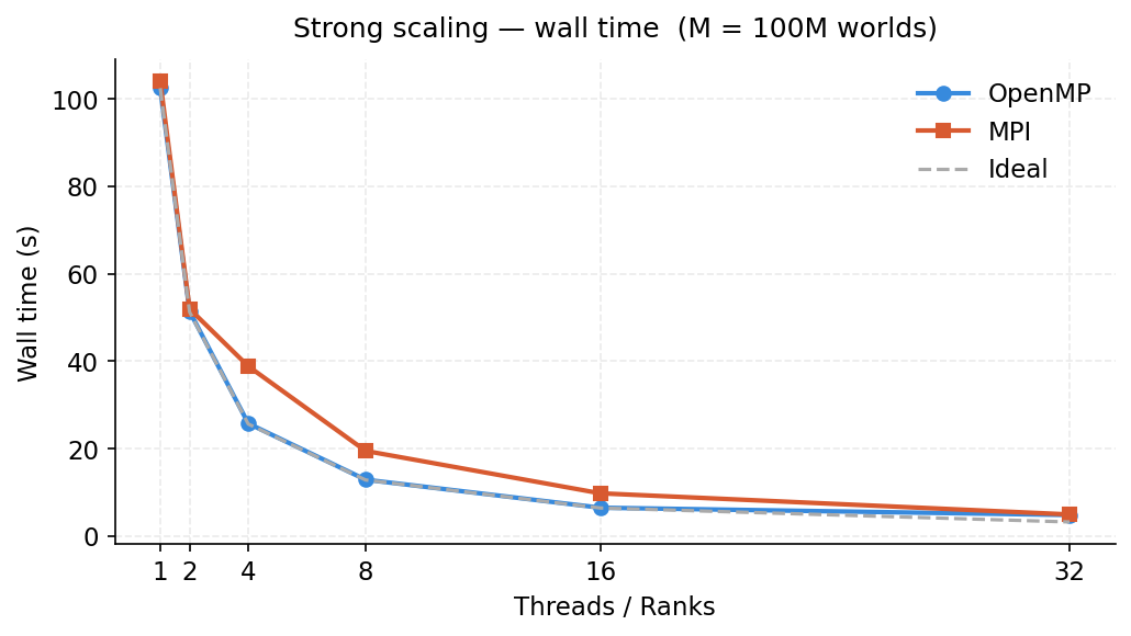Figure 1: Wall time for 100M worlds as thread/rank count increases.

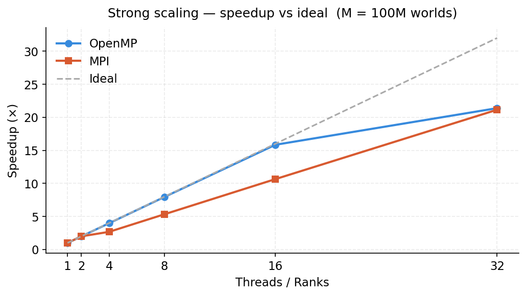Figure 2: Speedup relative to single-core serial baseline.

Strong scaling (M = 100M worlds):

Threads	Wall time (s)	Throughput (M worlds/s)	Speedup	P̂ (%)
1	102.462	0.976	1.00×	3.7227
2	51.405	1.945	1.99×	3.7227
4	25.749	3.884	3.98×	3.7242
8	12.873	7.768	7.96×	3.7222
16	6.466	15.466	15.85×	3.7216
32	4.791	20.871	21.39×	3.7237

Weak scaling (M = threads × 10M worlds):

Threads	M	Wall time (s)	Throughput (M worlds/s)
1	10M	10.275	0.973
2	20M	10.244	1.952
4	40M	10.304	3.882
8	80M	10.292	7.773
16	160M	10.302	15.531
32	320M	15.161	21.106

Both OpenMP and MPI achieve near-ideal strong scaling up to 8 threads/ranks. At 32 workers both reach roughly 21× speedup (wall time ~5s). OpenMP consistently outperforms MPI at the same worker count because it avoids inter-process communication entirely.

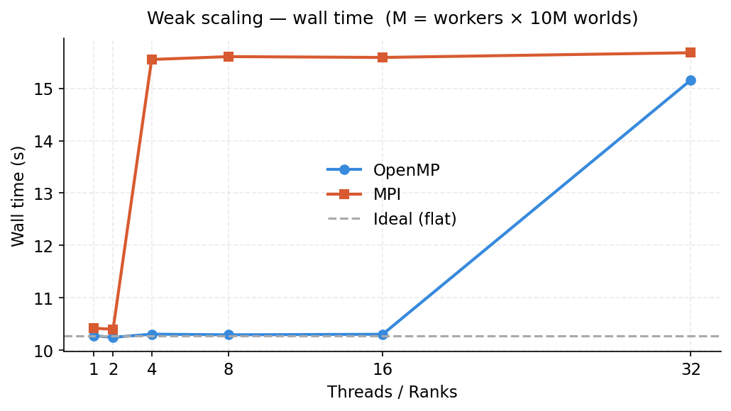Figure 3: Weak scaling — each worker processes 10M worlds, so total M grows with worker count.

MPI strong scaling (M = 100M worlds):

Ranks	Wall time (s)	Throughput (M worlds/s)	Speedup	P̂ (%)
1	103.966	0.962	1.00×	3.7227
2	51.956	1.925	2.00×	3.7227
4	38.840	2.575	2.68×	3.7242
8	19.462	5.138	5.34×	3.7222
16	9.759	10.247	10.65×	3.7216
32	4.917	20.337	21.15×	3.7237

MPI weak scaling (M = ranks × 10M worlds):

Ranks	M	Wall time (s)	Throughput (M worlds/s)
1	10M	10.418	0.960
2	20M	10.398	1.923
4	40M	15.553	2.572
8	80M	15.608	5.125
16	160M	15.592	10.262
32	320M	15.682	20.406

Weak scaling tells a different story. OpenMP stays essentially flat up to 16 threads (~10.3s), then rises slightly to ~15s at 32 threads as memory bandwidth pressure increases. MPI jumps immediately to ~15.5s at 4 ranks and plateaus there — the overhead is dominated by process launch and barrier cost rather than compute, so adding more ranks doesn't make it worse but the initial overhead floor is higher than OpenMP.

CUDA Performance

Run	M	Wall time (s)	Throughput (M worlds/s)	P̂ (%)	95% CI (%)
Correctness	10M	0.087	114.418	3.7243	[3.7126, 3.7360]
Benchmark	100M	0.855	116.898	3.7241	[3.7204, 3.7278]
Benchmark	1B	8.555	116.887	3.7213	[3.7202, 3.7225]
Benchmark	10B	85.545	116.897	3.7211	[3.7208, 3.7215]

Throughput is ~116.9 M worlds/s across all M values, meaning the kernel is fully saturated from 100M worlds onward. At 10B worlds the 95% CI narrows to just ±0.0004 pp. The CUDA implementation achieves a 180× speedup over the serial baseline.

JAX Performance

JAX was used to price all four contracts across both CPU and GPU backends. Unlike the other implementations which priced a single contract, JAX's vectorized kernel prices each contract independently in a separate timed run.

CPU backend (M = 100M worlds):

Contract	P̂ (%)	Naive (%)	Adjustment (pp)	Wall time (s)	Throughput (M worlds/s)
US invades ∧ Regime falls ∧ No nuclear deal	3.7218	2.8495	+0.872	45.086	2.2
Iran nuke ∧ NPT withdrawal ∧ No US invasion	0.3345	0.3282	+0.006	45.320	2.2
Full de-escalation: nuclear deal ∧ Hormuz normal ∧ No invasion	14.9613	12.4339	+2.527	45.002	2.2
Regional war: invasion ∧ Hormuz disrupted ∧ Kharg Island lost	4.0766	2.1220	+1.955	45.044	2.2

GPU backend (M = 1B worlds, NVIDIA L4):

Contract	P̂ (%)	Naive (%)	Adjustment (pp)	Wall time (s)	Throughput (M worlds/s)
US invades ∧ Regime falls ∧ No nuclear deal	3.7214	2.8495	+0.872	36.389	27.5
Iran nuke ∧ NPT withdrawal ∧ No US invasion	0.3346	0.3282	+0.007	35.946	27.8
Full de-escalation: nuclear deal ∧ Hormuz normal ∧ No invasion	14.9565	12.4339	+2.523	35.863	27.9
Regional war: invasion ∧ Hormuz disrupted ∧ Kharg Island lost	4.0787	2.1220	+1.957	35.982	27.8

On GPU, JAX achieves ~27.8 M worlds/s across all four contracts — about 4× slower than the CUDA kernel on the same hardware. On CPU, JAX at 2.2 M worlds/s is faster than the serial baseline (0.64 M worlds/s).

Profiling

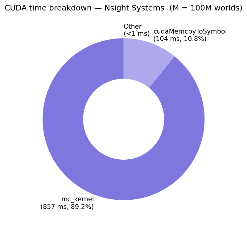Figure 4: CUDA runtime breakdown from Nsight Systems (M = 100M worlds).

Nsight Systems shows that 89.2% of GPU time is spent in mc_kernel (857ms) and 10.8% in cudaMemcpyToSymbol (104ms) — that's the one-time upload of the Cholesky factor to constant memory. The kernel is fully compute-bound.

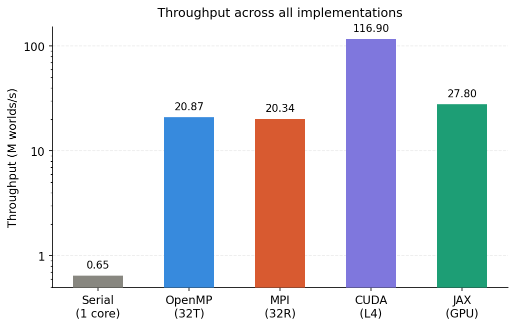Figure 5: Peak throughput across all five implementations (log scale).

Conclusion

This project implemented a correlated Monte Carlo contract pricer across five parallel programming models, using real Polymarket data for 33 Iran/Middle East geopolitical events. The simulation is embarrassingly parallel by nature since each world is independent, so it's really nice for testing parallel code.

The key finding from the simulation is that the correlated probability of the target contract (US invades Iran ∧ Iranian regime falls ∧ no nuclear deal) is 3.72% — meaningfully higher than the naive independent estimate of 2.85%, a +0.87 pp adjustment driven by the positive correlation between a US invasion and Iranian regime change.

And also we're doomed because everyone's addicted to sports betting, bye.